2: Equations and limits

Equations

To predict the course of mixing-limited reactions using a closure model, we will integrate differential equations for the average amount of the i-th species versus time:

\[\frac{d\overline{C_{i}}}{dt}=\sum_{j}{\nu_{ij}r_{j}}\]

where $\nu_{ij}$ is the stoichiometric coefficient of component i in reaction j (negative for reactants and positive for products). In a CFD context, the left hand side would be the substantive derivative. The average rate of the j-th reaction is given by:

\[r_{j}=k_{j}\overline{\prod_{i} C_{i}^{o_{ij}}}\]

where $o_{ij}$ is the order of species i in reaction j, that is the exponent in the rate law.

The closure problem for fast reactions between two separate streams arises because we do not know the (product of the) instantaneous concentrations needed to calculate the average reaction rate.

Mixture fraction and limits

To address this gap, the statistics of turbulent fluctuations in concentration, that is the temporal fluctuations at a fixed location, require estimation/ modeling. The combustion community and later Baldgya and others use the concept of mixture fraction and its variance to represent the fluctuations. Mixture fraction is a conserved scalar with value 1.0 in stream 1 and 0.0 in stream 2. When there is no chemical reaction, the relationship between species concentration and mixture fraction is given by the “mixing line” for each species, shown here for species in our 5-reaction azo-coupling example at typical concentrations - A is fed in stream 1 with B and C fed in stream 2:

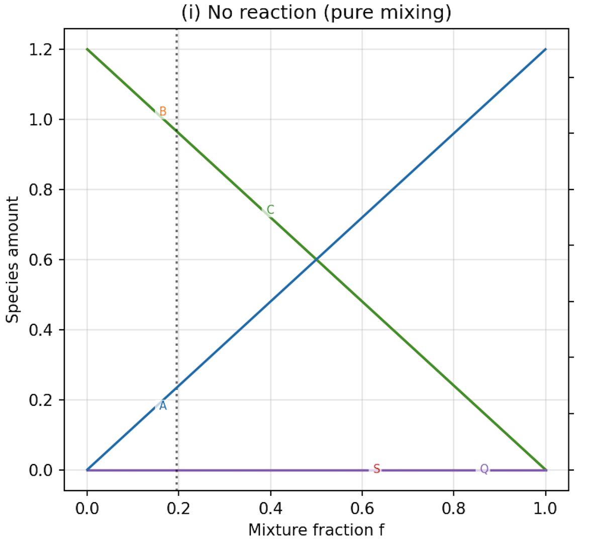
Turbulent fluctuations in the local value of f may be described statistically using the mean and variance of f and the beta proability density function (pdf) is a good representation that is commonly used (see more below). When the streams first meet, the variance is total, with essentially no contact with molecules from the other stream; in this case the beta pdf is like two delta functions at f=0 and f=1. The variance is reduced by mixing on various scales, in a cascade from larger to smaller eddies; as variance reduces, the pdf develops into a single broad peak, gets tighter and eventually becomes a delta function at the mean of f, corresponding to a completely mixed system with no concentration fluctuations. The mixing-sensitivity of chemical reactions occurs when the reactions are fast enough to take place at least partially while mixing is still in progress.

The mixing line allows calculation of the number of molecules (or moles) of each substance that would be present at any location if no reaction had occurred. That is one extreme limit that approximates the situation when the kinetics of all reactions are very slow. There is another extreme that describes behaviour when kinetics are infinitely fast; in that case, reactants from the streams cannot co-exist, as any collision between molecules would lead to immediate reaction.

For the 5-reaction version of azo-coupling, the reactions and kinetics (all in SI units) are as follows:

"reactions": [
  "R1: A + B -> R",
  "R2: A + R -> S",
  "R3: A + B -> T",
  "R4: A + T -> S",
  "R5: A + C -> Q"
  ],
  
  "rate_constants": {
    "R1": 12238,
    "R2": 1.835,
    "R3": 921,
    "R4": 22.25,
    "R5": 124.5
  },

For the 5-reaction azo-coupling with all reactions assumed to be instantaneous and taking place together:

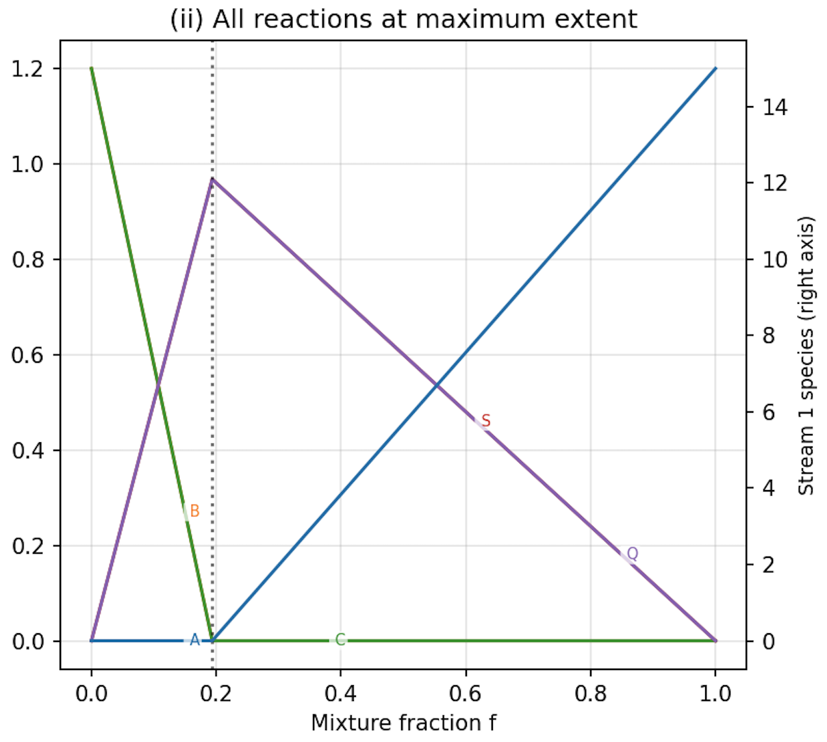
At this particular limit, A cannot co-exist with either B or C; and neither R nor T may be found in the product solution as both are immediately converted to S. The value of f at which this occurs is known as $f_{s}$, the “stoichiometric mixture fraction”. The profiles of products at this limit generally take the shape of a “tent” with a peak directly above $f_{s}$.

Baldyga’s closure equation

Baldyga’s 2009 and 2025 proposed closures estimate C(f) for any species based on interpolation between the mixing line and a limiting case with infinitely fast kinetics, using the average species concentration as a weight, or to interpolate between the limits:

\[C_{i}(f) = C_{i}^{\infty}(f)+[C_{i}^{0}(f)-C_{i}^{\infty}(f)]\frac{\overline{C_{i}}-\overline{C_{i}^{\infty}}}{\overline{C_{i}^{0}}-\overline{C_{i}^{\infty}}}\]

This results in something like the blue shaded line C(f) below for component C in the Bourne reaction, interpolating between the mixing line (shown dashed below) and an infinitely fast reaction limit (coloured black below); this snapshot plot was taken during simulation of the 5-reaction system:

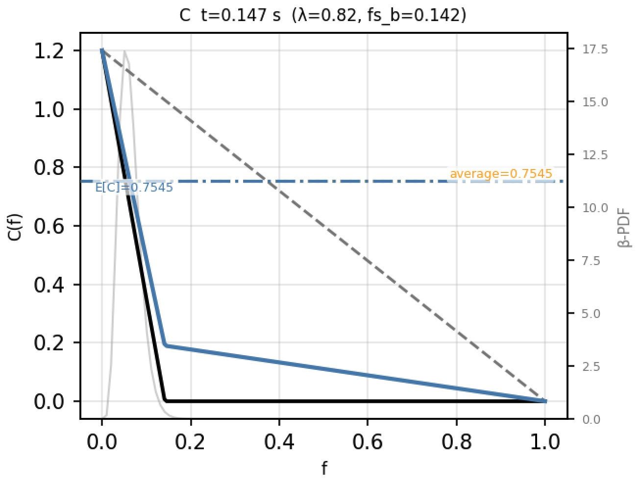
This plot also shows the beta pdf (in very light grey), centred around the average f of 0.0625 in this example, with values on the secondary y-axis. The pdf takes on a near-normal distribution as mixing proceeds towards completion. The dashed flat lines on this plot is the average concentration from the ODE solver and (not visible underneath it) the beta-integrated C(f). The labels on either side of the flat line are the numerical values of the average and beta-integrated C(f); in a mathematically and physically consistent closure, these should always be identical.

Estimating the average reaction rate

Once we have an estimate of C(f) for each species from such a closure, the average rate of reaction can finally be calculated using the pdf of f, representing the statistical behaviour of the instantaneous concentrations, as:

\[r_{j}=k_{j}\int_{0}^{1}{\phi(f) \prod_{i} C_{i}(f)^{o_{ij}}}\]

Note that in this product of concentrations we are obtaining the average product of typically two species concentrations (sometimes more). For each species, the closure provides C(f). The mixture fraction and its variance together with the bera pdf provide the statistical information needed about the concentration fluctuations. When integrating with CFD, a transport equation for f and each of the three contributing variances should be solved as part of Baldyga’s Turbulent Mixer Model, as described in his group’s publications. In my 2026 computations, I have used the analytical solution for variance provided by Baldyga’s group to calculate versus time (equivalent to downstream distance) in a plug flow system.