4: Baldyga's limits and my test set-up

Tests

The way to test closures is to solve the equations that use the closures and compare the results with reality (experimental data), other closures and references. As part of my open source species_limits.py project, I included the CVODE integrator from the excellent ¹ scikit-sundae library to solve the ODEs for each species. I used the same mixing parameters and calculations as the 2025 paper from Baldyga’s group, including the analytical solution for intensity of segregation, allowing the variance of f to be calculated easily at each time (or position). I also included the ability to perform an epsilon “sweep” from very slow mixing (1.0E-6 W/kg) to very fast mixing (1.0E+6 W/kg) with the same fixed reaction kinetics. That allows exploration of any closure over the full range of mixing timescales from almost completely segregated reaction conditions through to almost completely well-mixed reaction conditions. We are looking for closures that behave correctly at both ends of this spectrum and especially in the middle where both mixing and kinetics are influential and interact strongly. Each integration proceeds to 99.9% consumption of the limiting reactant; that is A in this case, fed through stream 1 where f=1. B and C are fed in stream 2 where f=0. The volume ratio of the streams is 15, so the mean of f is 1/(15+1)=0.0625. Feed concentrations (all $mol/m^{3}$ are 15, 1.2 and 1.2 for species A, B and C respectively. Both B and C are in overall excess compared to A.

Baldyga’s limits

Baldyga (1994) uses a closure interpolating between a pair of infinitely fast reaction subsets for both competitive-consecutive and competitive-parallel reactions. In the competitive-consecutive case, he discusses how $f_{s}$ moves as the product of the first reaction is produced and the second reaction is enabled to proceed. In the 2009 and 2025 papers from his group on the full 5-reaction system, the movement of $f_{s}$ is directly calculated from the amount of R (or S) already produced during reaction and interpolation is between the no-reaction limit and a combination of two infinitely fast reaction limits: subset numbers 20 and 31. Subset 20 contains reactions 1, 3 and 5 running infinitely fast; subset 31 contains all 5 reactions running infinitely fast.

Combination is a powerful idea as a means of identifying a unique infinitely fast reaction limit. If the right limit is calculated, C(f) for all species can then be obtained by interpolation between that (in this case, moving) limit and the no-reaction / mixing line.

I implemented this method as one closure option called “blend_fs” in species_limits.py. Full mathematical details of my implementation are available here. I tried to keep my implementation general and for example, did not rely on any reaction in any system being infinitely fast. I included an option for the user to stipulate/ hardwire precisely which reaction subsets to combine in the manner of the 2009 and 2025 papers; that enabled me to reproduce the method in the papers, I believe. (I am in contact with Magdalena Jasińska in Baldyga’s group and am checking and comparing computational details).

I stress that the following results are from the blend_fs closure in my implementation. This is intended to be identical to the closure described in the 2009 and 2025 papers from Baldyga’s group. Results using blend_fs will be compared later with Figure 11 b) in the 2025 publication. The results are very similar but not yet identical.

Simulation results using blend_fs

Simulations produce a wide array of plots that became important at various times during this work. Only a few plots are needed to extract the main results; other plots are helpful to perform reality checks and notice or diagnose problems with the model or the integration of the ODEs. Non-smooth behaviour in plots usually indicates a problem. Not all of the plots will be described here, you can generate them all if you run the code, but the main ones are as follows. These were obtained using epsilon=1 W/kg.

Profiles for species amounts versus time full-size:

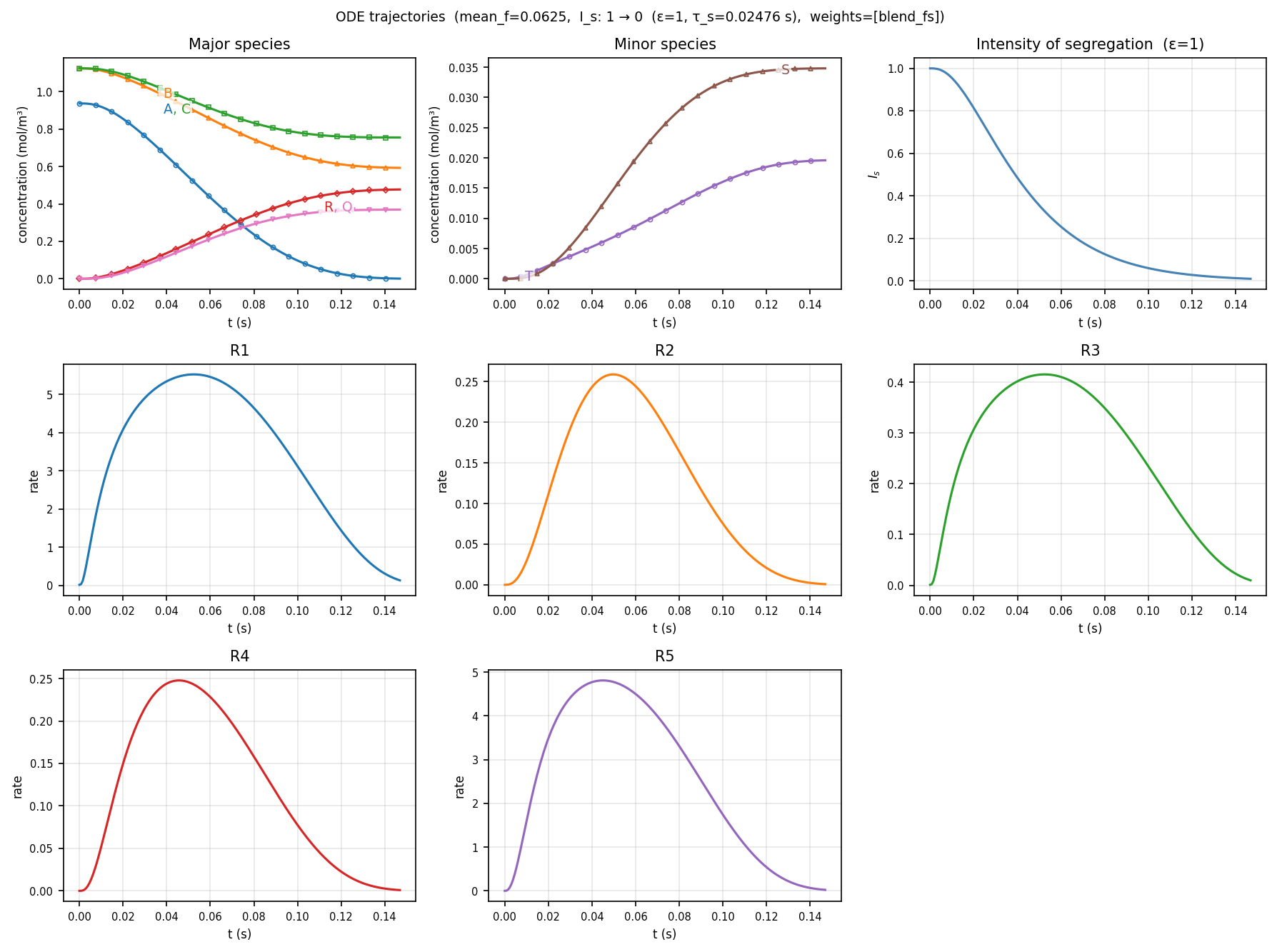
When running blend_fs (or any one closure) alone, this set of plots includes coloured subplots for major and minor species, a subplot of Intensity of segregation and finally subplots showing each of the reaction rates, all versus time.

Snapshots of C(f) for each species at several times along the reaction trajectory full-size:

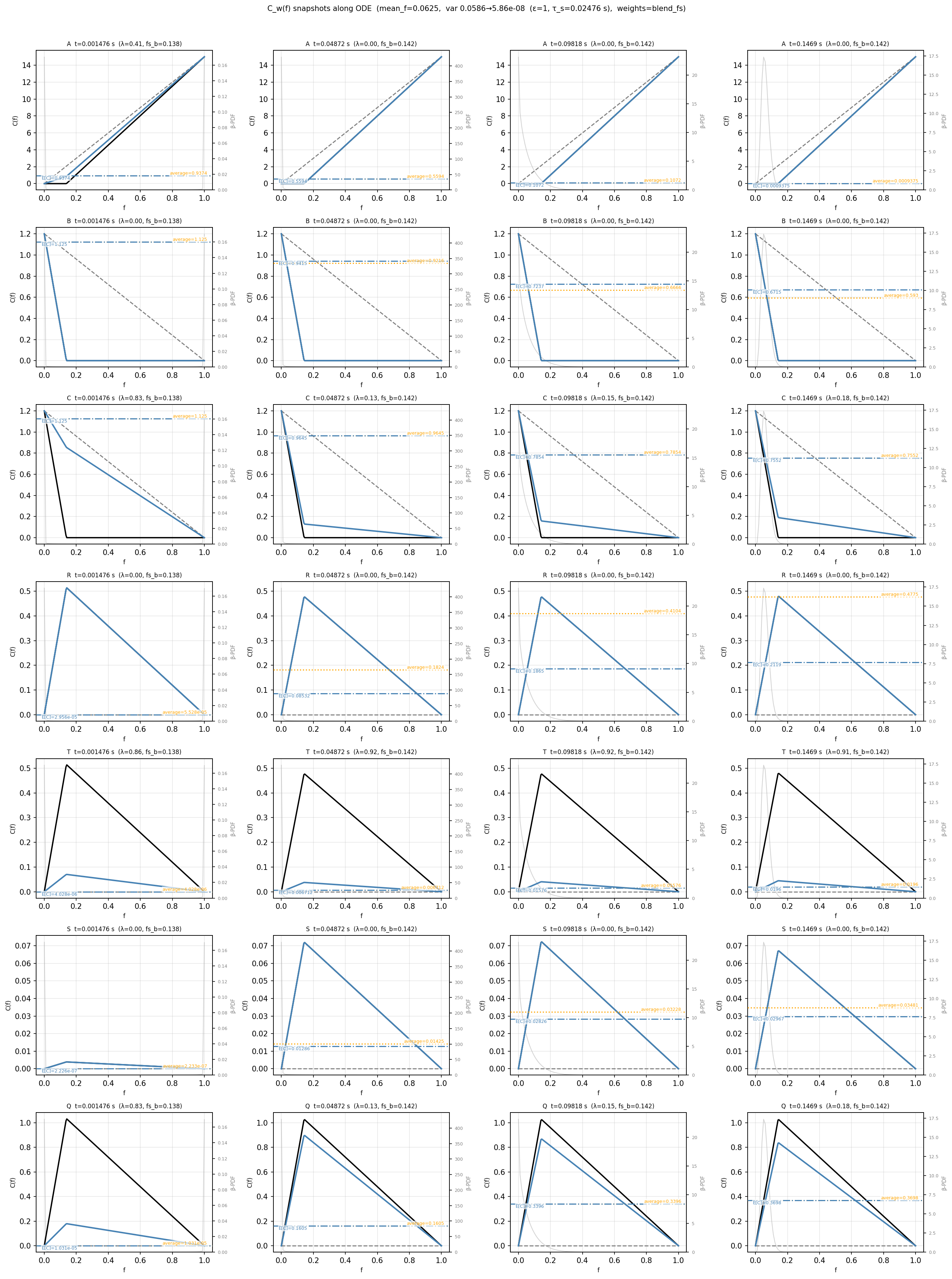
When running blend_fs alone, this array of plots show each species in its own row and each snapshot time in its own column. The timing of the snapshots in the first column is about 1% of the reaction time; the other three columns are equally spaced along the reaction time. Mixing (no-reaction) lines are dashed, and infinitely fast reaction lines are in bold black, with navy lines showing the interpolated C(f). Flat lines on each plot indicate the average concentration from the ODE and the beta-averaged C(f), which should agree with each other. Where two flat lines are visible, the average species concentration lies outside the pair of limits defined by blend_fs and the reaction rate is “clamped” to stay just within those limits; clamping reflects an internal inconsistency in the closure under clamped conditions. Clamping may lead for example to unexpected changes in the shape of reaction rates that are not physical.

Profiles of the beta-averaged values of all known limits, compared with the species amounts from the ODE solution full-size:

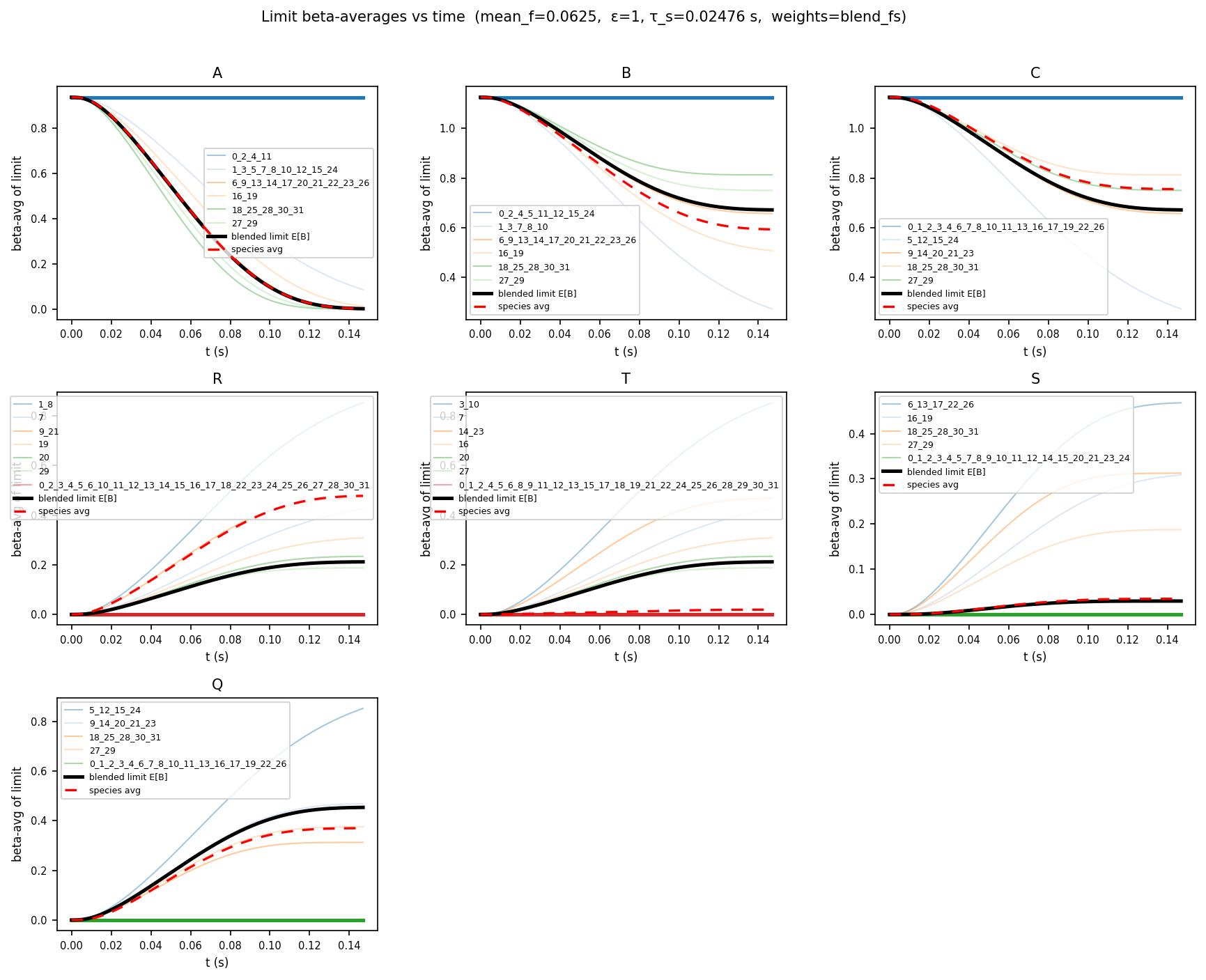
Here we have a subplot for each species versus time. The ODE trajectory on these plots is shown as a dashed red line; the other curves are the positions of the beta-integrated averages of the known limits for that species. The labels of the known limits comprise the reaction subsets for which that curve is the correct limit, with undercores between the identifiers of each subsets. Some curve labels are long because the species limit is the same for many subsets. The heavy black line is the beta-averaged combined limit calculated by blend_fs. When the ODE trajectory strays outside the range between the beta-averaged no-reaction limit (plot label contains 0) and the beta_averaged blend_fs moving limit, the solution is said to “clamp”, see above. That occurs in this illustration especially for components B and R.

When running blend_fs, we generate snapshot plots showing the evolution of (the moving) fs and the (changing) shapes of the “tent” plots for each species at the blend_fs combined limit full-size:

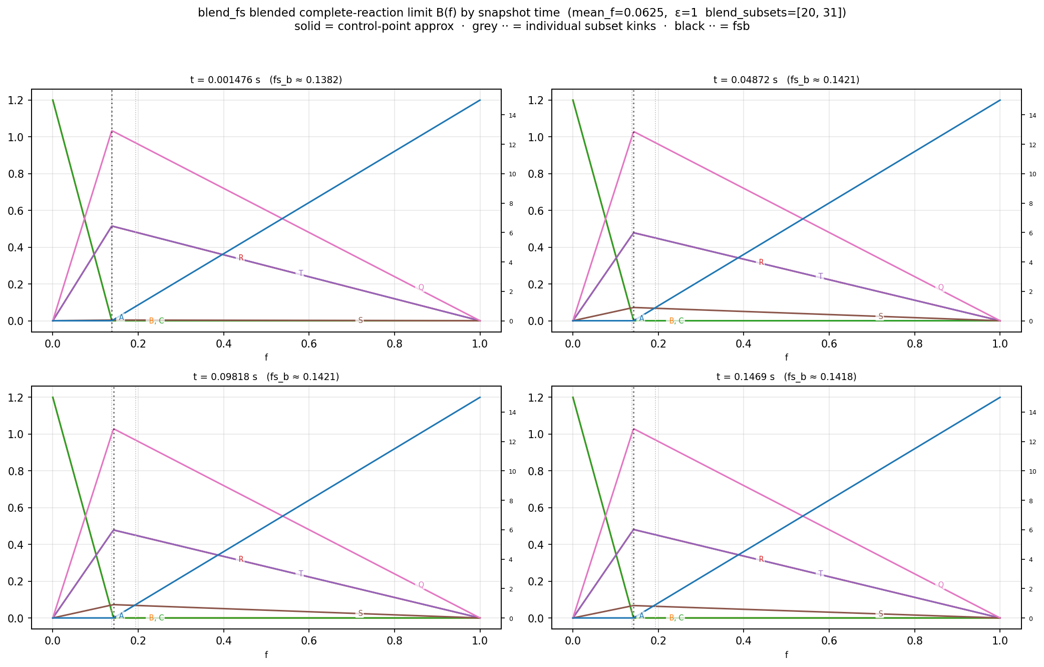
Once again, the timing of these snapshots is about 1% of reaction time and then equally spaced. In this case, fs does not change a lot when modeled using the closure from the 2009 and 2025 publications implemented in blend_fs.

When running blend_fs, we show the full evolution of (the moving) fs at the combined limit full-size:

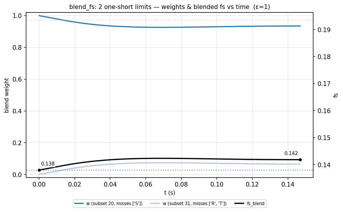
fs may not move much using blend_fs if the reaction conditions keep it near one of the boundary values; in this reaction system, there is most movement using blend_fs at low mixing intensity, where the amount of S produced during reaction is highest.

Product fractions versus time full-size:

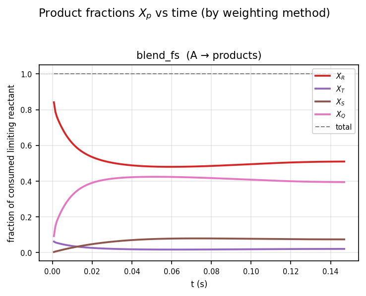
These plots show the evolution of the fractional product amounts made while consuming the limiting reactant; of particular interest are XQ and XS.

Results of an epsilon sweep full-size:

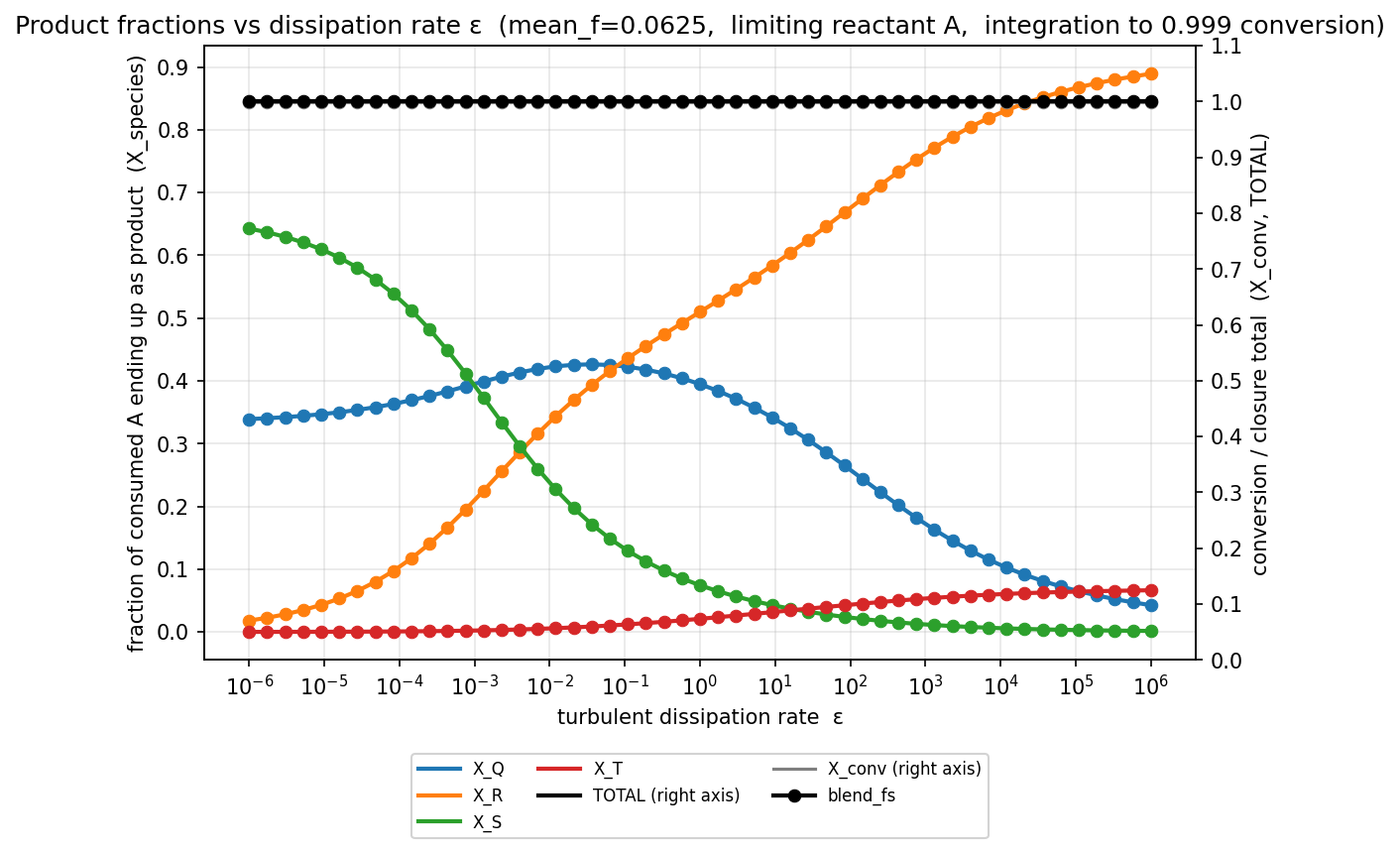
The epsilon sweep plot shows behaviour of the closure over a broad range of mixing conditions from very mild to very intense. At either end, XQ and XS tend towards limiting values corresponding with limitation by kinetics (at high epsilon) and mixing (at low epsilon).

Other diagnostics produced from a simulation include the CPU time (blend_fs is generally fast) and the number of times the ODE solution “clamped” C(f) to keep C(f) as used in the reaction rate calculation within the blend_fs pair of limits, even if the ODE solution average had driften outside those limits. The consequence of such a clamp is an internal inconsistency in the model, whereby the beta-averaged C(f) no longer equals the average calculated by solving the ODEs. That could lead to unexpected and likely unphysical changes in reaction rate during the simulations. We found that clamps were frequent for blend_fs and will discuss that more later.

Footnotes

1. scikit-sundae ↩