 Joe Hannon's blog
6: Other methods for bracketing C(f)
Motivation
For the 5-reaction azo-coupling there are 32 limits or 31 excluding the no-reaction limit. Blend_fs as described in the 2025 paper and previous posts uses only two of these 31 limits, in combination with each other. For general-purpose application of a closure, it is desirable to consider all of the limits as some may become relevant depending on kinetics, reactant amounts and mixing. This motivates the search for a general approach that in principle can adhere to any of the limits or a combination, depending on the current conditions; and that can be applied to any reaction scheme or system.
Linear interpolation between nearest limits
Idea: Baldyga’s closures use the average solution concentration to interpolate between pairs of limits. If the interpolation limits were closer together, it might be possible to obtain tighter bracketing and thereby a more accurate estimate of C(f). This might be achieved by considering all possible subsets and their limits and interpolating using the average concentration between the limits that most closely bracket the average.
Outcome: This method produces species and reaction rate profiles that are continuous but may contain abrupt changes as the bracketing limits change during solution of the equations. It never clamps. It produces the correct XQ and XS at either end of an epsilon sweep, but the XQ curve contains unphysical bumps at intermediate epsilon. It remains in the code as an illustration and a point of reference.
ODE solution at 1 W/kg compared with blend_fs full-size:
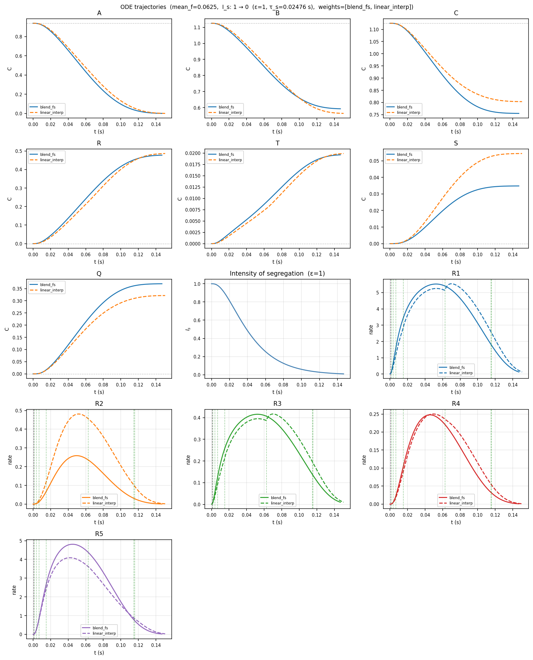
The linear-interp ODE solutions look similar to blend_fs but not identical by any means. The (busy) reaction rate plots show vertical lines ehere linear_interp has changed one of its pair of interpolating limits and some of these coincide with changes in the rate that are not physical.
Results of an epsilon sweep, compared with blend_fs full-size:
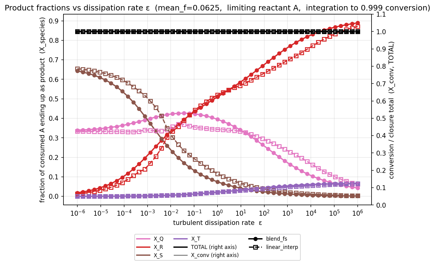
Linear_interp looks like it behaves correctly at each extreme of low and high epsilon, where it may be easier for it to find the right limit pairs. In the intermediate region, it is flatter and bumpier than the corresponding curves for blend_fs. It cannot capture the highest XQ values correctly and the bumps are not physical.
Linear interpolation between maximum and minimum limits
Idea: In order to give a closure maximum scope to “find” the right C(f) as it solves, one could use only the maximum and minimum limits for each species as bracketing values, ensuring where possible that the beta-averaged C(f) equals the average value from the ODE. By definition this method will not respect more than one correct fs limit at any time.
Outcome: Gave too much freedom to C(f) and left C(f) for some reactants well above zero at mixture fractions when it should be near zero. When two poorly bracketed profiles are cross-multiplied to get reaction rate, deviations from physical limits become pronounced. This method was not pursued.
Linear combination of all limits
Idea: In order to ensure that the closure keeps in mind all possible values of all limits at any time and might thereby “find” the correct limit, one could estimate C(f) as a linear combination of all of the limits based on the proximity of the species average value to the beta-average of each of those limits. A small iterative optimization (like sequential least squares, SLSQP) would be required to find the weights on each limit for each species.
Outcome: Produced C(f) line segments with multiple fs kinks and left C(f) for some reactants well above zero at mixture fractions when it should be near zero. When two poorly bracketed profiles are cross-multiplied to get reaction rate, deviations from physical limits become pronounced. This method was not pursued.
Variations of blended limits
Idea: One could generalize the Baldyga approach of blending a combination of subsets/limits. Possibilities include identifying subsets in any reaction system that are missing products and combining their limits based on the products they produce, to calculate a more general moving limit. When this specific (one short) idea was applied to the 5-reaction system, it used three limits (20, 27, 29) and did not select one of the limits used in the 2025 paper (20,31); that is because limit 31 is missing two products, R and T, rather than one product.
Outcome: An area worthy of some further investigation, especially if it is possible to find a general and automatable basis for selecting subsets to blend.
Results of an ODE solve, using blend_fs to automatically blend three limits (20, 27, 29) that are each one short of a product, compared to base case Blend_fs using subsets 20, 31 full-size:
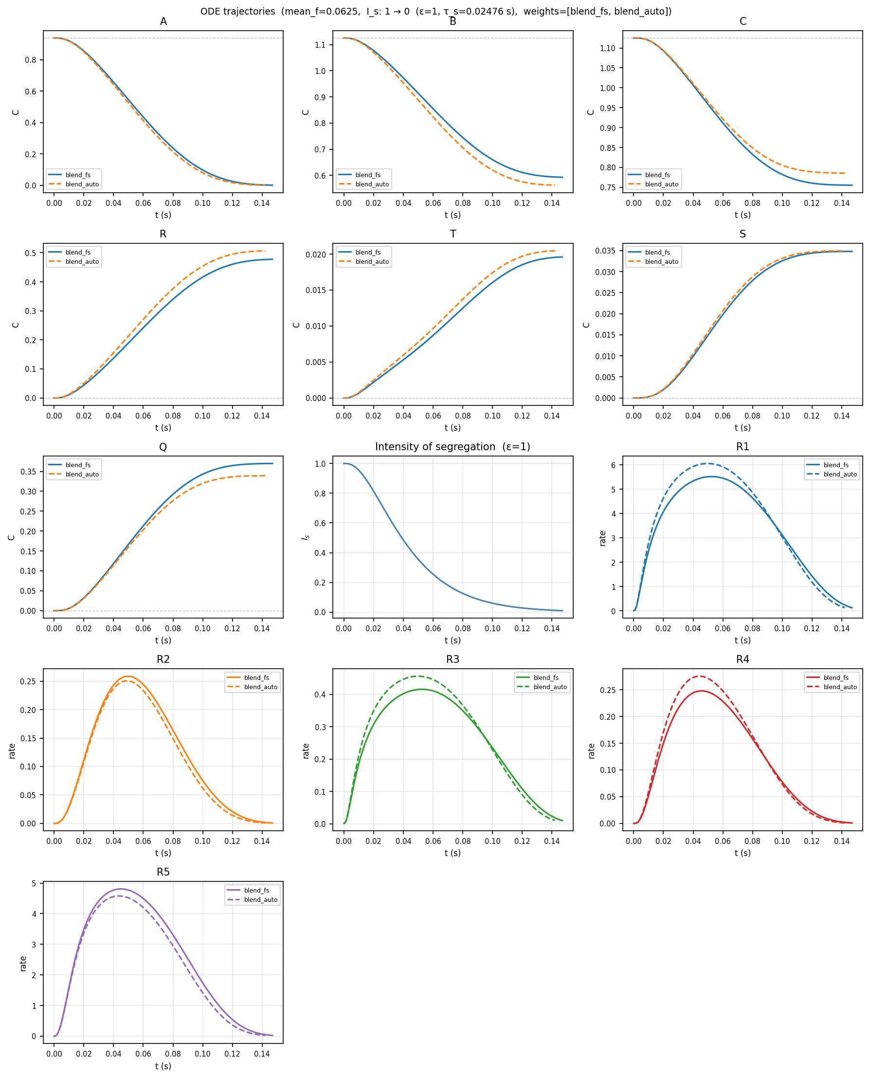
Under these conditions, the reaction rate profiles are smooth and well-behaved. Diagnostics generated during the solve continue to show significant clamping of the solution with subsets 20, 27, 29 (denoted blend_auto).
Results of the corresponding epsilon sweep full-size:
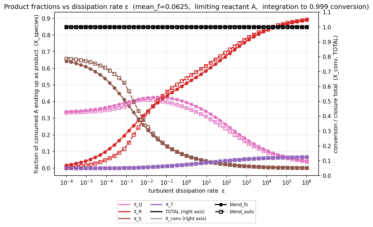
The fractional product curves such as XQ and XS with 20, 27, 29 (blend_auto) are generally quite smooth and behave well at either end.
With this particular blend_auto selection of subsets (20, 27, 29), XQ rises slower and then a little more sharply than it did using blend_fs (subsets 20 and 31). It is possible that with another basis for automated limit selection, results would be nearer to or even better than the results using subsets 20 and 31.