7: A new closure method: 'ray_limit'

A new closure method that appears to be generally applicable

It became clear when considering the various methods described in post 6 (and others) that if the profile of C(f) is not well-bracketed and respecting physical limits, closures will not work well. Hoping that the solution will “find” the right bracketing limits on its own from the precomputed static subsets is not realistic and additional information needs to come from somewhere in order to navigate subset-space and f-space. Rationally combined or blended and dynamic limits, such as those in the 2009 and 2025 papers from Baldyga’s group, looked more promising, although potentially internally inconsistent if the selected limits did not always bound the ODE average at all times. And it was not yet clear how such a combination could be determined and applied in a general or automatic way to a new and user-defined reaction system that differs significantly from the azo-coupling example we are using for illustration.

While thinking about the extra information that might help a closure to produce the correct solution in all cases, I often thought about how the kinetic parameters in the scheme contain useful information about which static limits might be most relevant to a solution. That is also true of the reaction conditions, especially the input concentrations of each substance, which determine to some degree what reaction pathways will be more active/relevant. None of the closures tried so far have made automated use of this information. In a bit of a light-bulb moment, I realized that it should be possible to extract from the ODE (or CFD) solution, which reflects all of these inputs, a trajectory that could be useful in defining the overall direction of the reactions in stoichiometric terms.

A mechanistically correct reaction system containing multiple reaction lines can be written in a single line that is stoichiometrically correct, even if the chemistry does not take place mechanistically in a single step. In fact, much traditional experimentation on reaction kinetics applies a similar idea when focused on determining the reaction order for each reactant.

I decided to use the ODE solution to determine the stoichiometric coefficients in that overall reaction and then push (or scale) conversion of the overall reaction to maximum extent based on the reactants currently available. The idea was that this would form a single limit that represented a dynamic combination of subset limits from the static set and would bound C(f) on one side while the mixing line would bound C(f) on the other. In principle this method would always ensure that the beta-integrated mean equalled the ODE average, with no clamping, as the maximum extent limit would by definition always be further along than the current extent. A nice advantage was also that it was not necessary in this method to even compute all of the subsets up front, although that is advisable and informative. Crucially, the method could be automated easily to apply to any reaction system and was not restricted in any way to specific types of chemistry. And it was not restricted in any way to a particular pair or set of $f_{s}$ values; instead, it determined its own $f_{s}$ depending on the progress of the particular reactions being simulated and all of their kinetic parameters and reaction conditions.

I called this method “ray_limit”, because in mathematical terms it is extracting from the ODE solution a “ray” (or vector/arrow) that points in the direction in which the overall chemistry is moving. When there are $N$ reactants and products, there are $N$ components in the ray. I found some ways to visualize it in geometric terms and watch how it changes e.g. during reaction; it turns out that $f_{s}$ is quite sensitive to any shift in the ratios of the ray components. A detailed mathematical description of ray_limit is provided here.

Implementation in code is quite simple and generic, with a fresh infinitely fast reaction / maximum extent limit being calculated from the current ray at each integration step and used together with the mixing line and the species average from the ODE to interpolate C(f). When I saw how well this worked, it was quite exciting, as it offered for the first time the possibility to apply appropriate and well-behaved closure models for C(f) to any chemistry in an automated manner.

Simulation results using ray_limit

Once again, we compare key results with blend_fs (which uses subsets 20 and 31).

ODE solutions compared at epsilon=1 W/kg full-size:

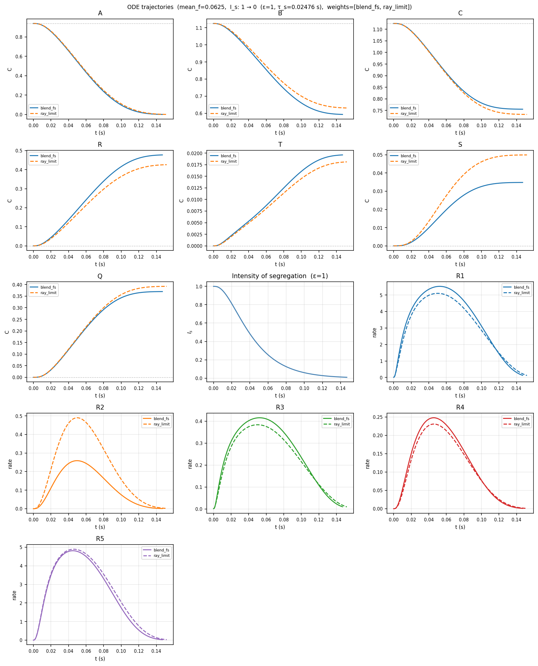
The ODE solutions look quite similar overall with both methods under these conditions, but are not identical. Reaction rates in general are subtly different and R2 is noticeably higher with ray_limit under these conditions.

Results of epsilon sweep full-size:

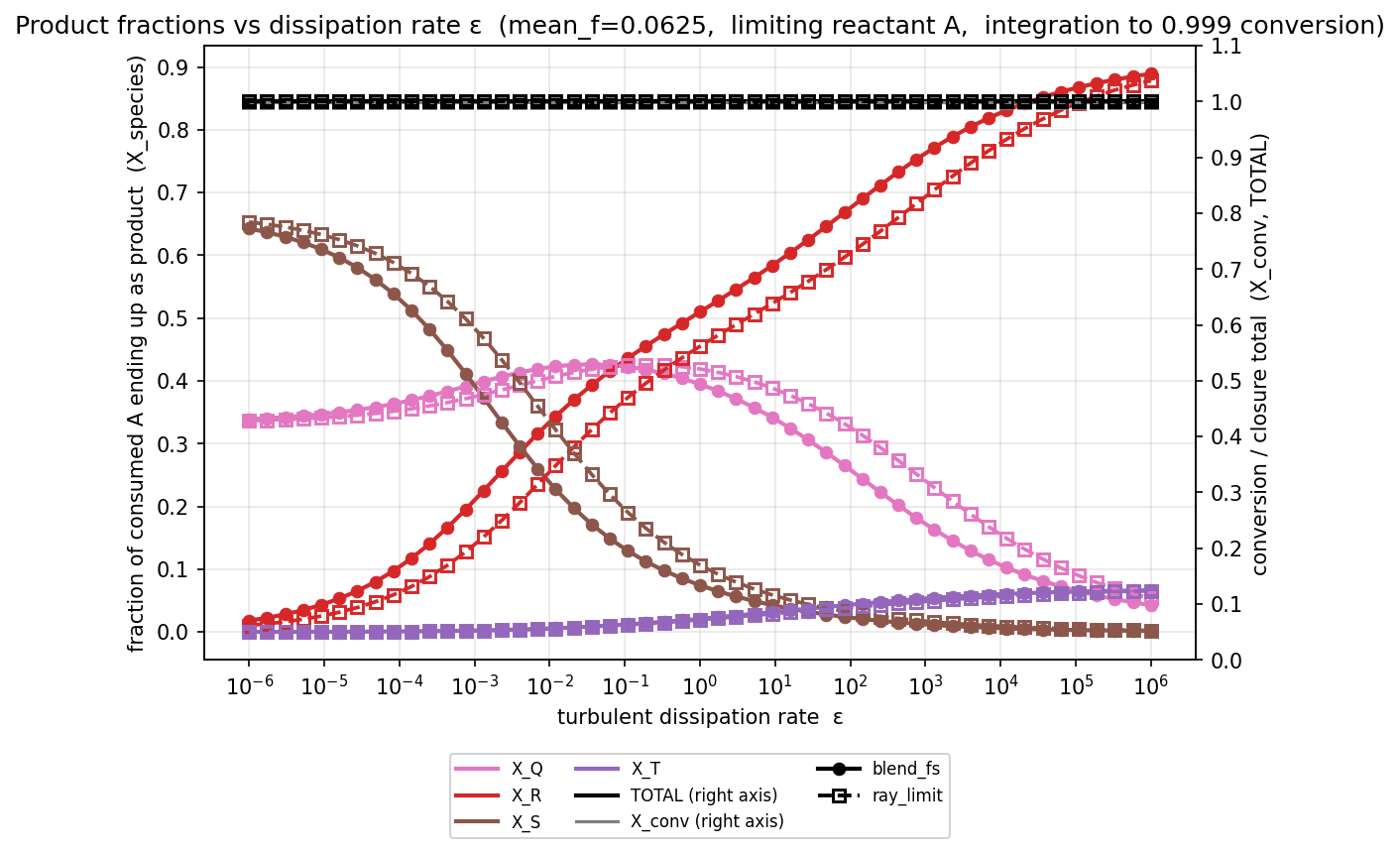
Both methods produce XQ and XS curves with similar smooth shapes that behave correctly at the extremes. ray_limit calculates higher values of XS at low epsilon and higher values of XQ at higher epsilon.

A significant difference between ray_limit and blend_fs is that ray_limit does not “clamp” during the ODE simulation, that is the beta-average of C(f) never strays outside the limits. For blend_fs, e.g. at epsilon=1 W/kg, species B and R both clamp with blend_fs and the following plot illustrates and compares the behaviour with species B.

Comparing the ODE solution with the beta-averages of the limits full-size:

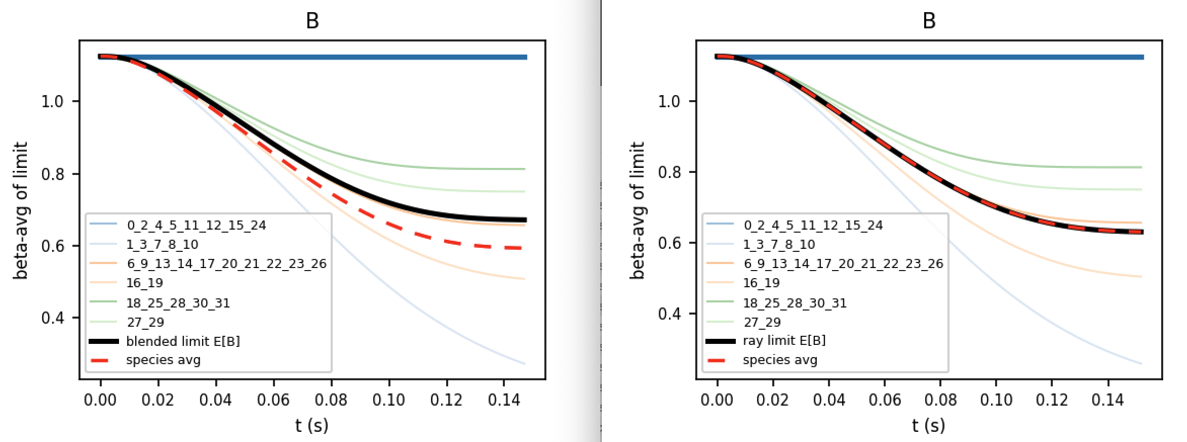
The general behaviour of both methods and their differences will be discussed in the following posts.