 Joe Hannon's blog
9: Comparison of results with 2025 paper
Basis of overall comparison
I have used Figure 11 b) from the 2025 paper as the main basis for comparison of overall results. This shows final product fractions (or distibutions) versus epsilon over the range 1.0E-6 W/kg to 1.0E+6 W/kg. I have separately overlaid results for XQ and XS using blend_fs (plotted using dot symbols) and using ray_limit on the results with the full closure model in the 2025 paper (plotted using solid lines). The dashed lines shown are from the original Figure 11 b) and relate to calculations using a simplified version of Baldyga’s closure; the dashed lines may be ignored for the purposes of the present discussion.
blend_fs results compared with 2025 paper
Results from an epsilon sweep using blend_fs, compared to Figure 11 b) in the 2025 paper full-size:
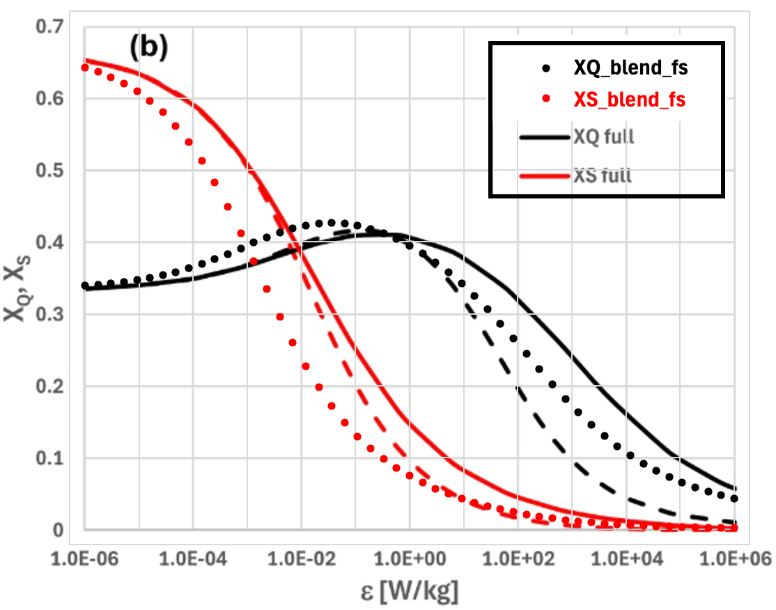
The shapes of the curves from blend_fs (dotted) and the 2025 paper (solid) are very similar and generally the curves are close to each other and approach each other at both ends. (At the left end, mixing is almost fully rate-controlling and at the right end, kinetics are almost fully rate-controlling). There is a clear offset in the x-direction (epsilon), with the blend_fs peak in XQ occurring at a lower epsilon; XQ values are initially higher on the left, but XS values are lower and the net effect is that mixing appears “better” with blend_fs. The same type of offset persists at higher epsilon, with blend_fs giving XQ values that are below the 2025 paper. It is reasonable to think on this basis that in my blend_fs implementation, mixing is somehow more effective than in the 2025 paper’s implementation. More information on possible implementation differences is given below and I am in discussion with Baldyga’s group to clarify those differences.
ray_limit results compared with 2025 paper
Results from an epsilon sweep using ray_limit, compared to Figure 11 b) in the 2025 paper full-size:
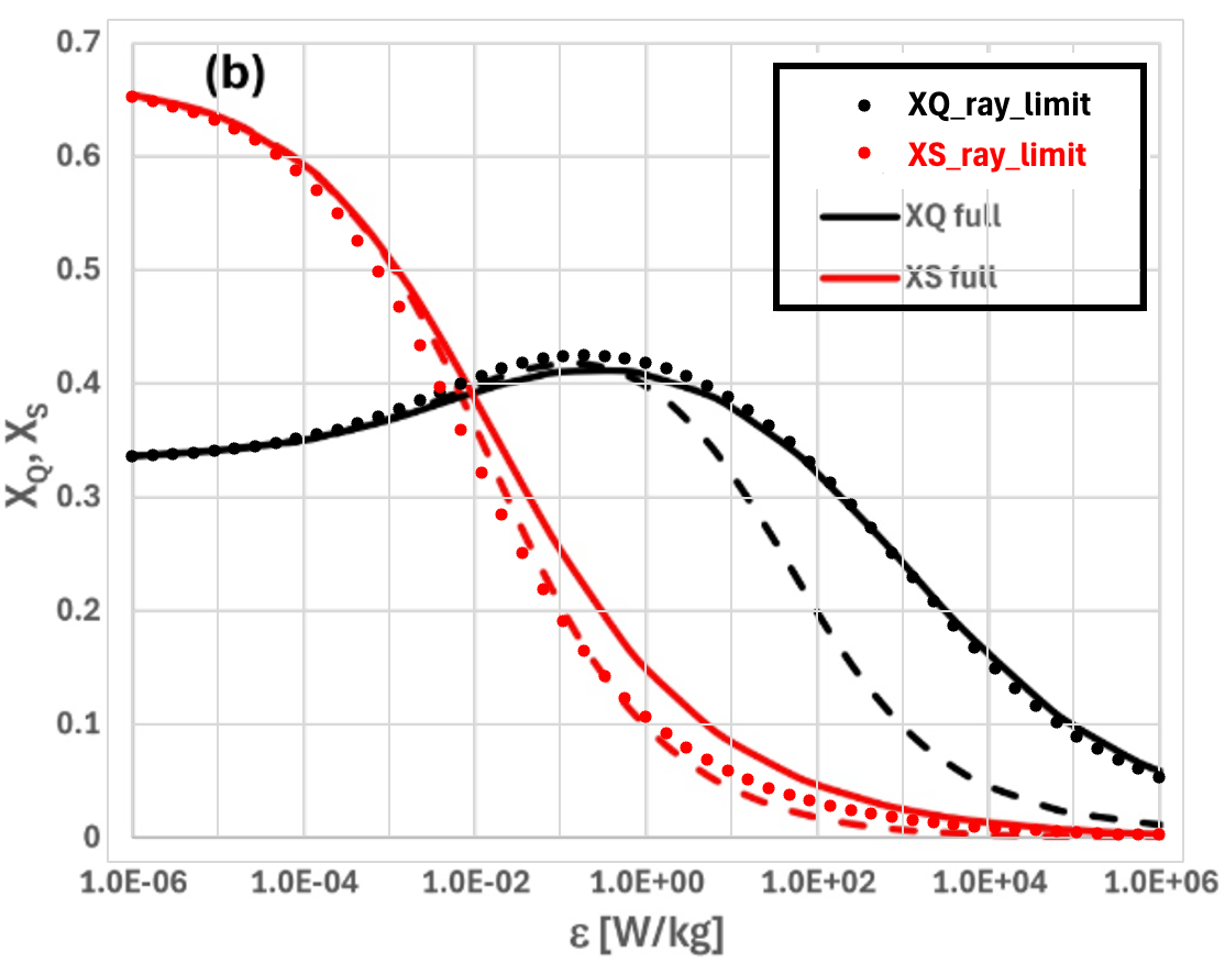
The shapes of the curves from ray_limit (dotted) and the 2025 paper (solid) are even more similar than the curves for blend_fs above and generally are closer to each other and approach each other more tightly at both ends. There is a small offset in the x-direction (epsilon) with XS values a little lower with ray_limit than in the 2025 paper. ray_limit and the 2025 paper (as well as blend_fs) use different closure methods to estimate C(f) and I expect this to be the major reason for any differences in these curves. On the other hand, the similarity between ray_limit results and the 2025 paper is notable.
Possible reasons for differences
The following are potential differences in implementation between the 2025 paper and blend_fs:
- Mixing parameters relating to Figure 11 b) are calculated differently; mixing (or more accurately variance) in these closure models is calculated from Intensity of Segregation. I have checked that my code produces exactly the same Intensity of segregation profile as in Figure 4 a) of the 2025 paper when the same input values are used for the integral scale of turbulence ($\lambda$, $\nu$ and $Sc$):
–
m_lambda=0.006 m_nu=1.0E-6 m_Sc=4000 - XQ and XS are calculated differently; I calculate XQ and XS after 99.9% conversion of the limiting reactant; I do not know at what point these are calculated in the 2025 paper
- The ODE solvers are different; my ODE simulations use the CVODE BDF stiff solver, with tight tolerances to ensure accurate integration
_ODE_RTOL = 1.0e-8
_ODE_ATOL = 1.0e-10
; I do not know what ODE solver or tolerances are used in the 2025 paper - The kinetic parameters are different; I use the kinetic parameters from Section 2.0 in the 2025 paper; no reactions are assumed to be infinitely fast
- The ODEs solved are different; I solve all of the species ODEs in their dimensional and untransformed state; the 2025 paper solves the ODEs in dimensionless form
- If/when the ODE solution average drifts outside the calculated limits, this is handled differently; I set the reaction rate to use C(f) at the limit that has been breached. I call this “clamping”. I do not know if/how this is handled in the 2025 paper
- My calculation of the moving fs in blend_fs and the corresponding species concentrations C(f) is different to the beta-based reaction calculation in the 2025 paper (Equation 41 in the 2025 paper); I have checked the values produced by Equation 41 are identical to those in my blend_fs implementation (see plot below)
- Reaction rates weighted by the beta function pdf are calculated differently; I use the Scipy betainc function to integrate the piecewise linear C(f) functions in closed form, with no quadrature truncation error. I do not know how the beta function is integrated in the 2025 paper
- My calculations to date have been on Apple Silicon; I do not know the compute architecture used for by the 2025 paper.
Plot of of $C_{R}(f)$ and $C_{S}(f)$ as calculated using blend_fs, at discrete values of beta (the ratio of S to (R+T+S)) full-size:
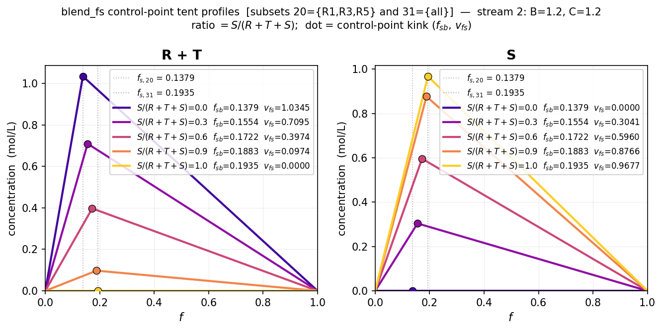
The values of $f_{s}$ and the concentrations correspond exactly with calculations by hand using Equation 41 from the 2025 paper; the concentrations correspond exactly with those presented in dimensionless form in Figures 6 and 7 of the 2025 paper.
I will report here when we know more about which of the above listed potential reasons or some other reasons explain the small differences between my implementation of blend_fs and the 2025 paper. I would like to compare my blend_fs results against the full results of ODE simulations using the code that generated the plots in the 2025 paper, that is the profiles for all species versus time, the intensity of segregation and the reaction rates, over a range of epsilon values.
In subsequent posts I will discuss some fundamental differences between the new ray_limit closure and the blend_fs / 2025 closure. I will illustrate those discussions with results generated by my implementations of both blend_fs and ray_limit.