10: Differences between blend_fs and ray_limit

I will discuss here some fundamental differences between the new ray_limit closure and the blend_fs / 2025 closure. I will illustrate those discussions with results generated by my implementations of both blend_fs and ray_limit. Then I show that an extended version of the 2025 closure behaves better than blend_fs and agrees exactly with ray_limit.

Clamping

During integration of the ODEs using blend_fs, the ODE solution deviates from the limits defined in blend_fs (aligned with the 2025 paper). We can see that in the evolution of the average species profiles (red dashed line) versus time when overlaid with the current values of the limits (bold curves) full-size:

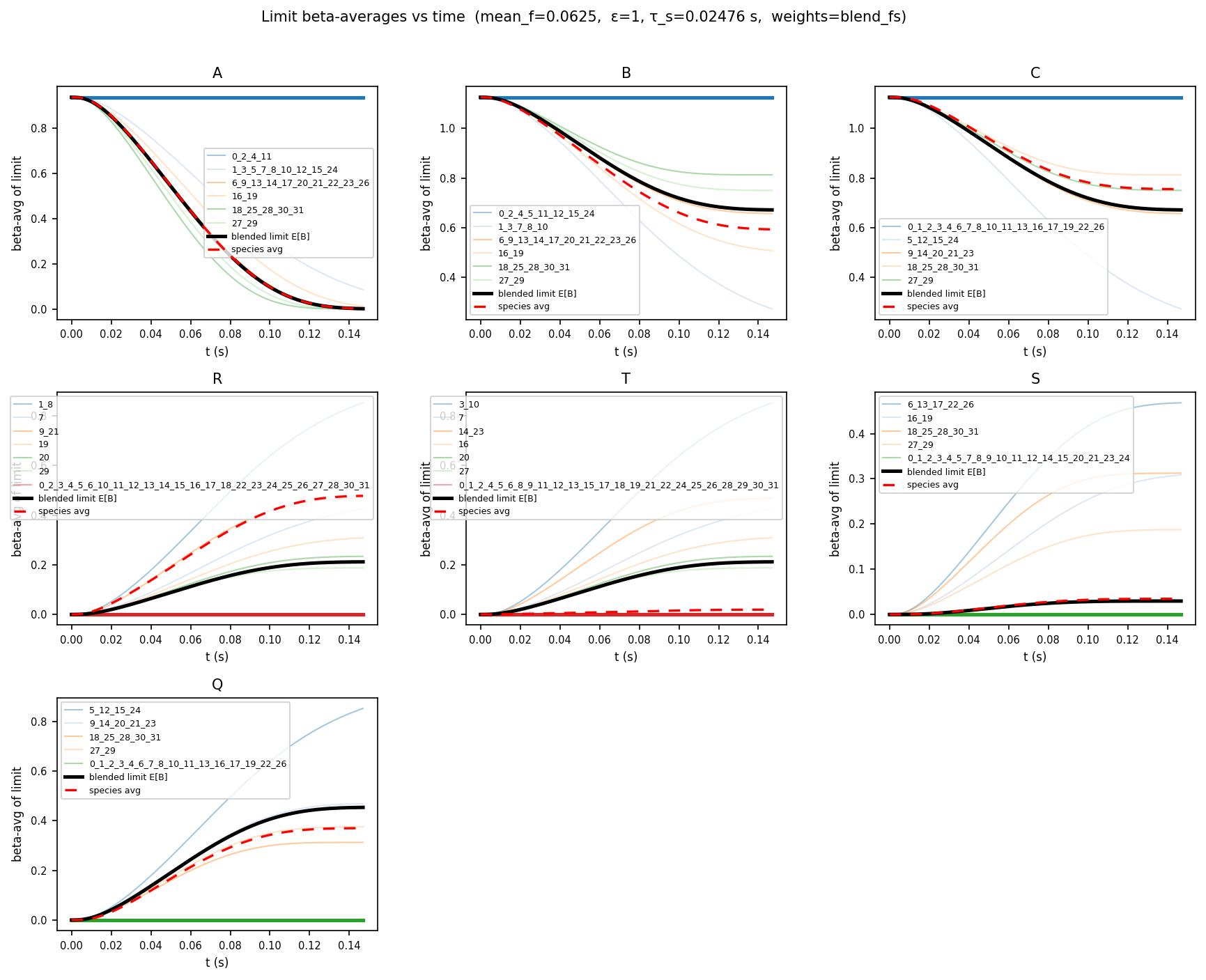
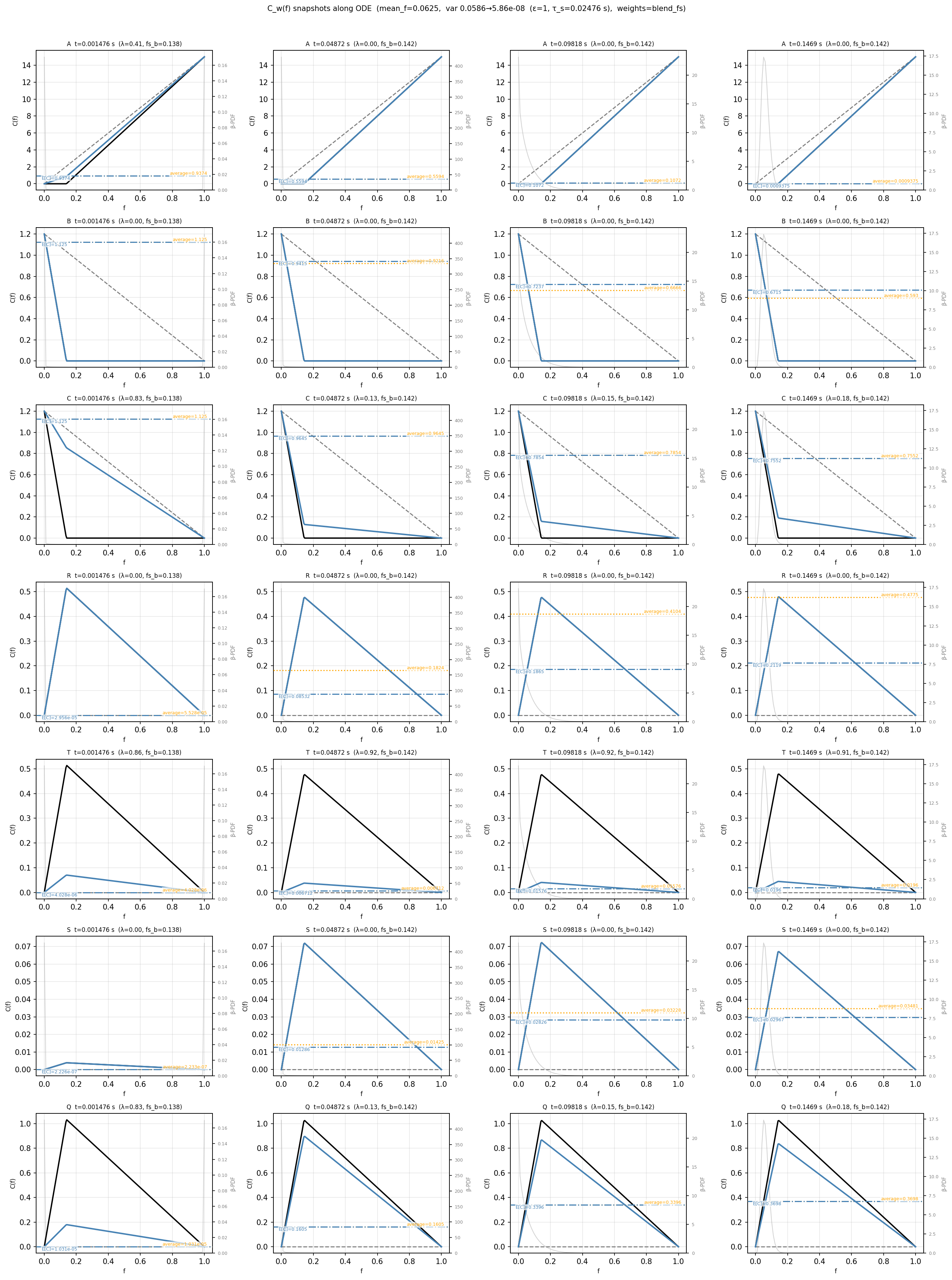
In the above plots, B and R clearly clamp/ stray outside limits. This is also evident in snapshot plots of C(f) in which the ODE solution (flat line) does not always equal the beta-averaged C(f); that is because I clamp C(f) to remain at the physical limit even if the ODE solution has gone outside that limit full-size:

I generate plots showing the percentage of ODE timesteps for each species that were clamped with blend_fs full-size:

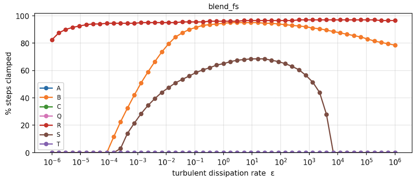
Clamping occurs to a significant extent over the whole range of epsilon and is most prevalent for species B and R (S is not relevant to calculation of rates in this example).

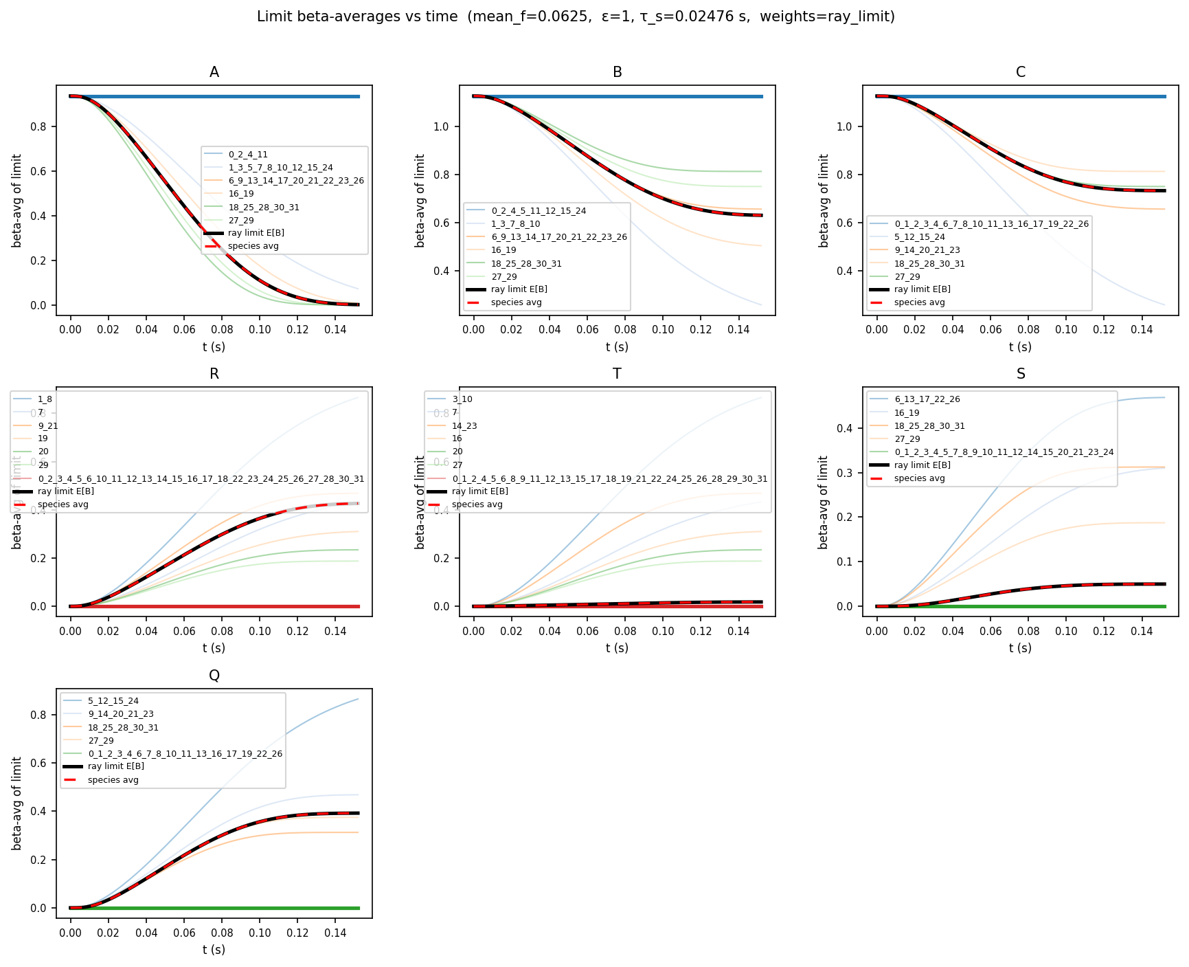
Clamping does not occur when using ray_limit in this example and in most other practical cases I have studied. Clamping is avoided using ray_limit by definition / by construction. The infinitely fast reaction has always proceeded further along the ray than the current reaction with finite kinetics full-size:

Position of fs

blend_fs calculates the current (moving) fs from limits 20 (fs=0.1379) and 31 (fs=0.1935), the same limits referenced in the 2025 paper. I generate plots of the evolution of fs versus time (black curve, secondary y-axis) in each ODE solution when using blend_fs full-size:

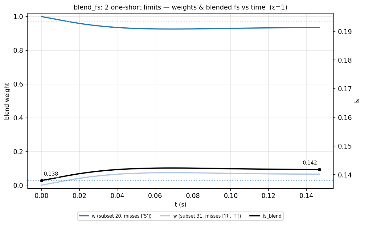
I also generate plots of the final fs at each epsilon during an epsilon sweep full-size:

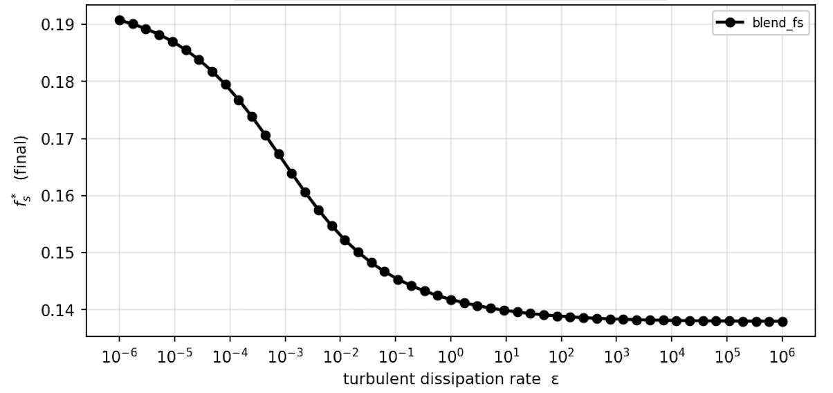
It is clear that fs moves from near 0.1935 at low epsilon, reflecting slow mixing and high production of S, towards 0.1379 at intermediate and high epsilon, reflecting faster mixing and less production of both S and Q.

I believe that in this example, fs need to be allowed to move across a wider range than this, as with increasing epsilon, reaction 5 is no longer behaving similarly (in terms of speed) to reactions 1 and 3, with more R and T and less Q being produced. I believe that additional limits should be considered in this closure that allow A and B to react more preferentially towards R and T than towards Q. In my terminology, those would be limit 7 (fs=0.0741) especially and possibly also limit 26 (fs=0.1379).

I also plot the evolution of fs (black curve, secondary y-axis) during simulation when using ray_limit full-size:

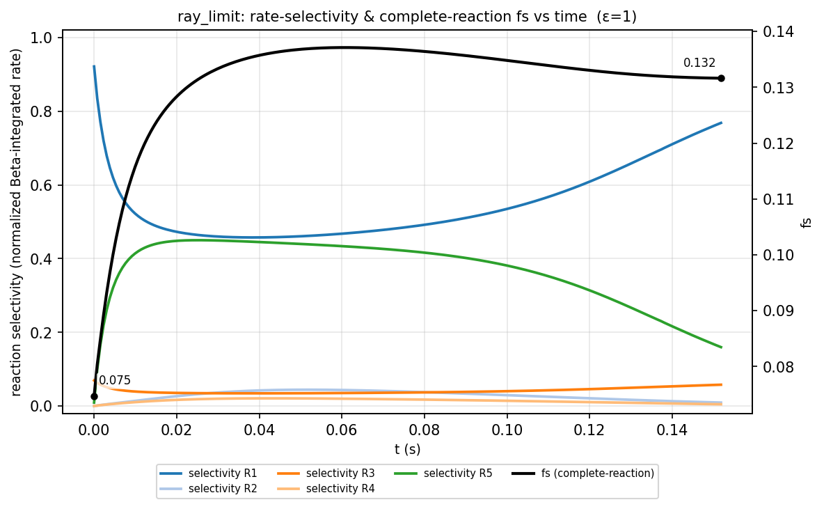
It is clear that ray_limit starts under these conditions at a lower fs than blend_fs can do and then varies significantly and smoothly as the reaction proceeds. The “selectivity” plotted on the main y-axis is a normalized version of the rate of each reaction and shows the shift in the relative balance of the reaction rates versus time.

I have compared the variation of the final fs in each simulation during an epsilon sweep using ray_limit and blend_fs and it is clear that ray_limit allows fs to adopt a smooth variation from almost 0.1935 at low epsilon down to near 0.0741 at high epsilon full-size:

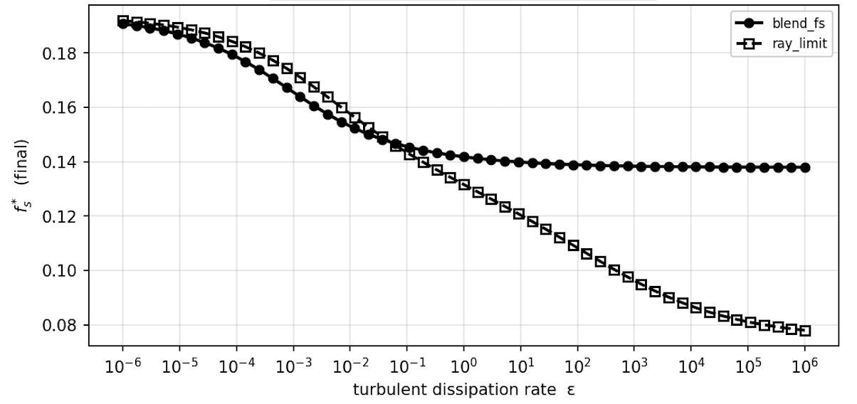
The evolution of fs using ray_limit is automatic and smooth and the limits do not even need to be calculated up front.